
[ad_1]
Google Sheets is a remarkably highly effective and handy instrument for gathering and analyzing knowledge, however typically it may be exhausting to know what that uncooked knowledge means. One of the most effective methods to see the massive image is to type it to assist convey crucial info to the highest, displaying which is the most important or smallest worth relative to the remaining.
It’s not shocking that Google Sheets has a robust search characteristic. It’s additionally simple to type knowledge in Google Sheets, however a number of ideas should be clear to realize the most effective end result and glean essentially the most useful insights. With a number of suggestions, you may rapidly grasp sorting by a number of columns and be capable of convey up completely different views for a greater understanding of what the information means.
How to rapidly type a easy sheet
Sorting a Google sheet by a single column is fast and simple. For instance, with a desk of meals which are good sources of protein, you may need to type by identify, serving dimension, or quantity of protein. Here’s how to try this.
Step 1: Move the mouse pointer over the column that you just need to type by and choose the Downward arrow that seems to open a menu of choices.

Step 2: Slightly over midway down the menu are the kind choices. Select Sort sheet A to Z to type all the sheet so the chosen textual content column is in alphabetical order. Sort sheet Z to A locations that column in reverse alphabetical order.
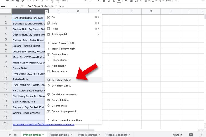
Step 3: To type a numerical column, comply with the identical process. Choose Sort sheet A to Z for a low-to-high order of numerical values or Sort sheet Z to A to see the best values on the prime.

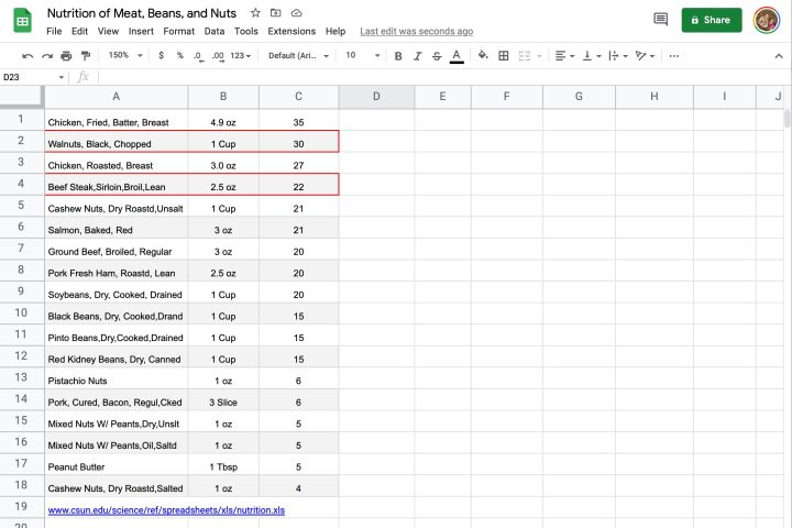
Step 4: No matter which column is sorted, the data from all different columns within the sheet is moved to maintain the identical order. In our instance, a cup of walnuts continues to point out as 30 grams, and a 2.5-ounce steak has 22 grams of protein.
Step 5: If a numerical column exhibits values in multiple unit, the kind will fail to present the anticipated end result. In our instance, the Google Sheet about protein sources, the serving-size column consists of cups, ounces, tablespoons, and slices. Units are ignored by the built-in type characteristic conversion, so 1 cup will incorrectly be handled as if it is smaller than 3 ounces. The greatest resolution is to transform the information to make use of just one unit per column.

Sorting a sheet with headers
The quick-sort methodology described above is handy; nonetheless, it would not work as anticipated when the sheet has headers. When you are sorting all the sheet, all rows are included by default, which might combine headings and models with the information. Google Sheets can lock cells to allow them to’t be modified, however it’s additionally doable to lock a number of rows in place on the prime so headers do not get confused together with your info.
Step 1: To freeze the place of header rows, select the Google Sheets View menu. Instead of utilizing your browser’s view menu, open the View menu on the prime of the online web page that is open. Then, choose the Freeze choice and select 1 row or 2 rows, relying on the variety of header rows in your sheet.
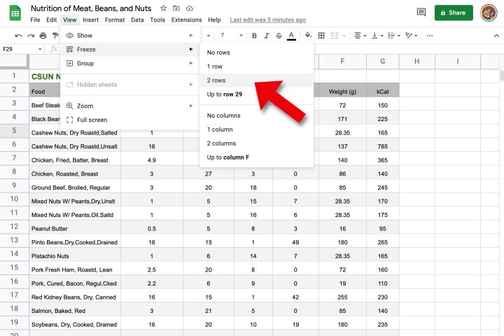
Step 2: If there are extra headers, it is doable to freeze extra rows. Simply choose a cell within the lowest header row, then select Freeze, then Up to row X within the View* menu, the place X is the row quantity.

Step 3: After freezing headers, a thick grey line seems to point out the place the break up happens. A sheet can then be sorted utilizing the column menu’s Sort sheet A to Z or Sort sheet Z to A choice. This leaves the headers in place on the prime of your Google sheet whereas rearranging your knowledge right into a extra helpful desk.

Sort by multiple column
A single-column type is fast and helpful, however typically, there’s multiple variable to contemplate when evaluating figures. In our instance, you is perhaps most by which has the least fats but in addition need to get extra protein. That’s simple to do with a kind vary.
Step 1: Select the cells that you just need to type, together with one header row. This might be finished rapidly by selecting the top-left cell, then holding down the Control key (Command key on a Mac) and urgent the Right arrow to pick the complete width of the desk.
Step 2: The similar might be finished by choosing the complete top, holding Control, and urgent the Down arrow. Now all the desk of knowledge will probably be chosen.
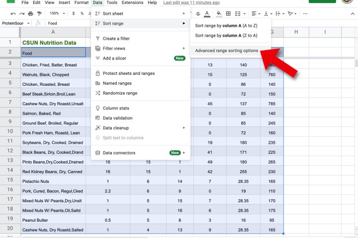
Step 3: From the Google Sheets Data menu, select Sort vary > Advanced vary sorting choices.
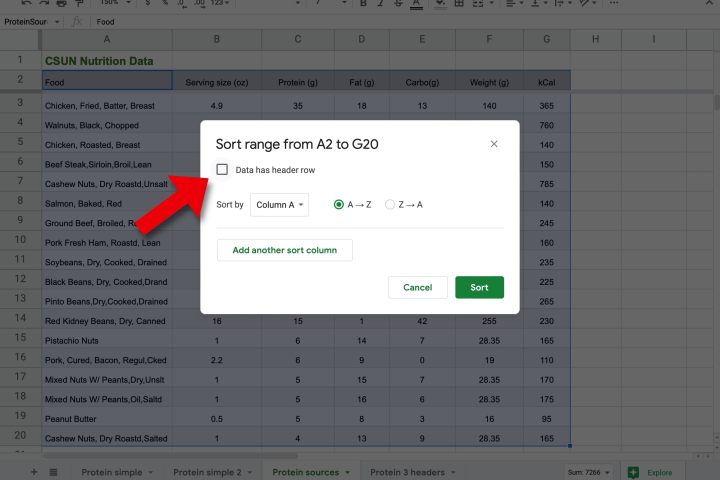
Step 4: A window will open that permits you to decide a number of type columns. If your type vary features a header row, test the field beside Data has header row.
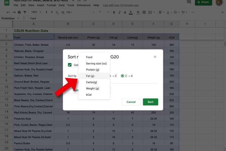
Step 5: The Sort by subject will now present your header column names as an alternative of constructing you select columns by utilizing their letter designation. Pick the first type column — for instance, Fat (g) — and ensure A-Z is chosen for type order.
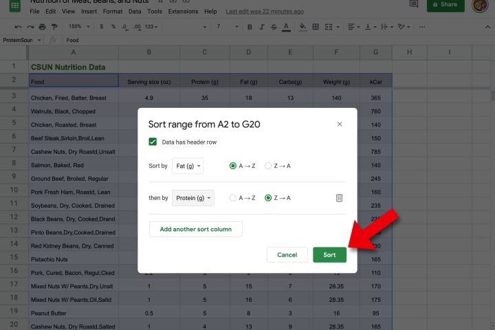
Step 6: Choose the Add one other type column button to have a secondary type, similar to protein. It’s doable so as to add as many type columns as you need earlier than choosing the Sort button to see the outcomes.
Save a knowledge vary
Instead of choosing a spread each time you need to re-sort it, it can save you the desk as a named vary.
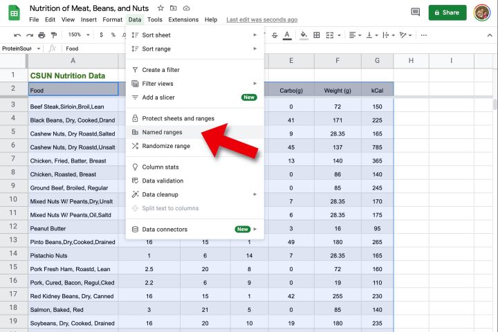
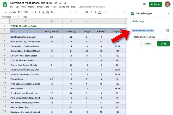
Step 1: Select the vary of knowledge that you just need to save for simpler entry, then select Named ranges from the Google Sheets Data menu.
Step 2: A panel will open on the best, and you may kind a reputation for this vary.
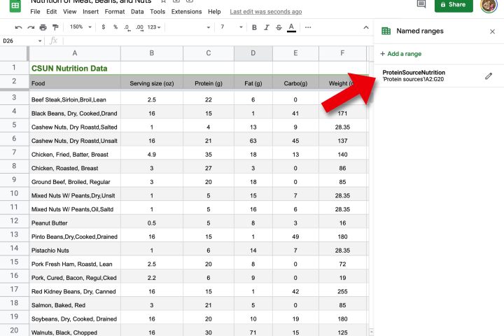
Step 3: The Named ranges panel will stay open, and you may choose all the vary once more by selecting it from this panel.
Saving a kind view
It’s additionally doable to save lots of multiple superior type operation for straightforward entry sooner or later. This permits you to change between completely different views when making a presentation or when it’s worthwhile to analyze info from completely different angles. This is feasible by making a Google Sheets filter view.
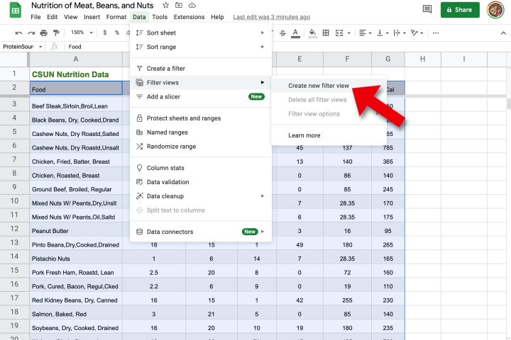
Step 1: Select the vary of knowledge you need to type, then select Create new filter view from the Filters submenu in Google Sheets Data menu.
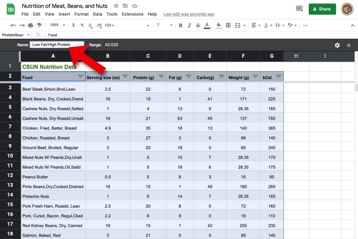
Step 2: A brand new bar will seem on the prime of the sheet with filter view choices. Choose the identify subject and kind a reputation for this filter view, similar to “Low Fat/High Protein.”
Step 3: The identify of every header column will now embrace a kind menu on the best aspect. Using our instance knowledge, select the Protein type menu after which choose Sort Z-A to put the best values on the prime.
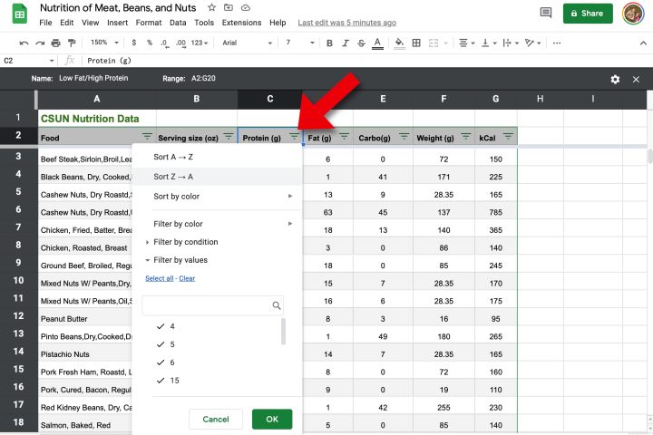
Step 4: Repeat this course of on the Fat type menu however select Sort A-Z to point out the bottom values first. This new filter view will present a kind with low fats being the highest precedence and excessive protein as a secondary consideration.

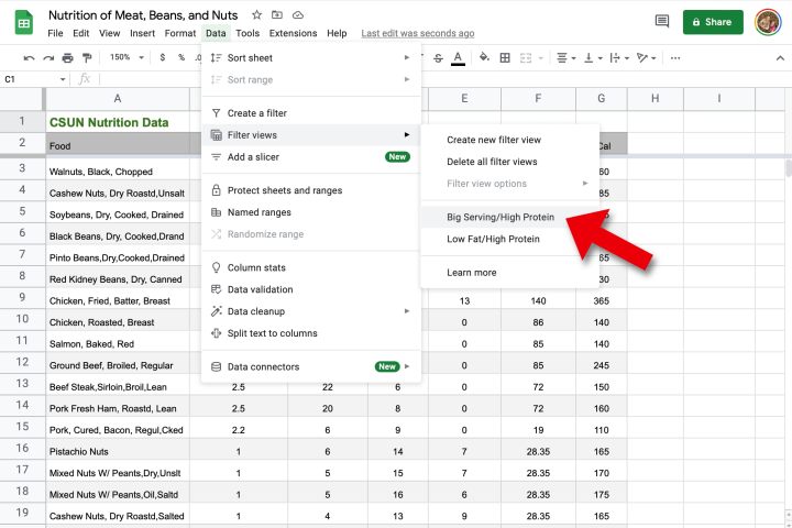
Step 5: You can create extra filter views in the identical approach and use as many type columns as wanted. To load a filter view, open the Data menu, choose Filter views, then choose the view that you just’d wish to see.
How to share a sorted Google Sheet
Google Sheets is available to anybody with an web connection, making this an incredible instrument for sharing info with others.
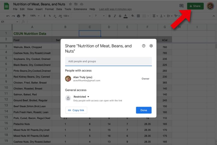
Step 1: Sorted spreadsheets might be shared by choosing the massive inexperienced Share button within the upper-right nook.
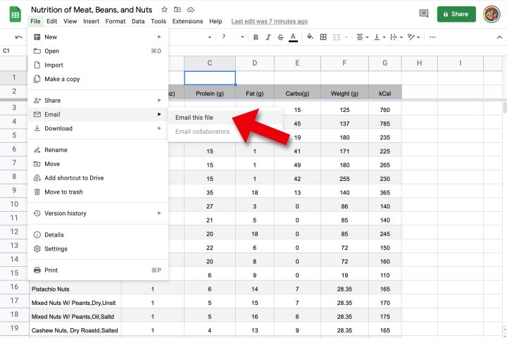
Step 2: It’s additionally doable to obtain a Google Sheet to share over e mail or print it to ship by way of common mail.
Google Sheets offers a number of methods to type knowledge, and this could make in massive distinction when making an attempt to investigate a sophisticated knowledge set. For extra info, try our full newbie’s information that exhibits use Google Sheets.
We even have a information that explains make graphs and charts in Google Sheets, a good way to see knowledge in an easy-to-digest visible type.
Editors’ Recommendations
[ad_2]